Why this matters: By 2026, the aquaculture engineering consensus is clear: the future of dissolved oxygen management is predictive, not reactive. Farms adopting hybrid AI-IoT platforms achieve 15–30% energy savings, 5–10% FCR improvement, and near-elimination of hypoxia-related mortality.

Why Dissolved Oxygen Prediction Modeling is Critical for Intelligent Aquaculture

From reactive to proactive: The paradigm shift in DO management

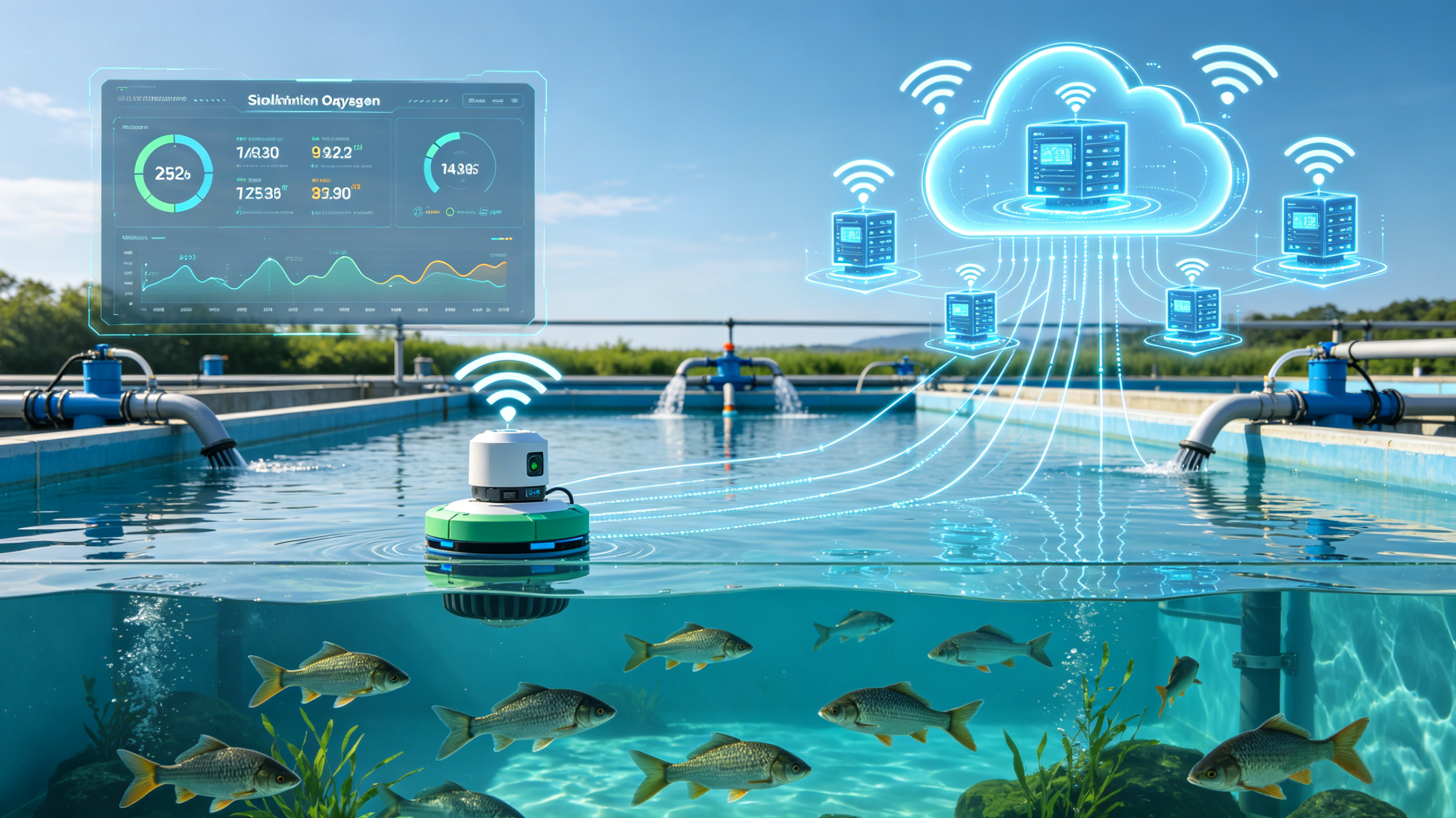
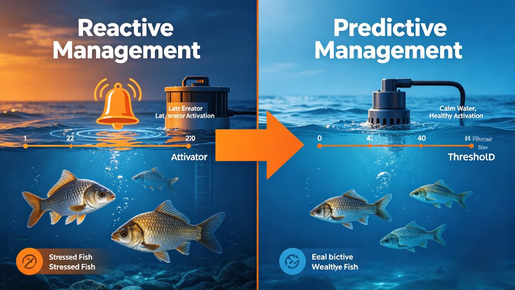
Dissolved oxygen prediction modeling enables a shift from reactive alarms to proactive control. Traditional dissolved oxygen (DO) management relies on threshold-based alarms: oxygen drops below 3 mg/L, aerators turn on. This reactive approach inevitably leads to stress, sublethal damage, or catastrophic crashes because DO dynamics are driven by nonlinear interactions—photosynthesis, microbial respiration, diurnal cycles, and sudden weather events. The paradigm shift toward predictive control uses historical and real-time data to forecast DO levels 30–120 minutes ahead, allowing preemptive aeration before critical thresholds are breached. Proactive management not only prevents mortality but also stabilizes the aquatic environment, reducing feed conversion ratio (FCR) volatility.

The economic impact of accurate DO prediction on FCR and survival rates

Quantitative evidence from controlled RAS and pond trials shows that accurate dissolved oxygen prediction modeling (R² > 0.85) translates into 5–10% improvement in FCR because fish maintain normal feeding behavior and metabolic efficiency. Hypoxic events trigger cortisol spikes, reducing growth rates and increasing disease susceptibility. For a 100-ton annual production farm, a 2% improvement in survival rate returns tens of thousands of dollars. Moreover, intelligent aeration reduces energy consumption by 15–30% compared to continuous or timer-based aeration, directly improving profit margins.

Enabling technologies: IoT sensors, cloud platforms, and AI

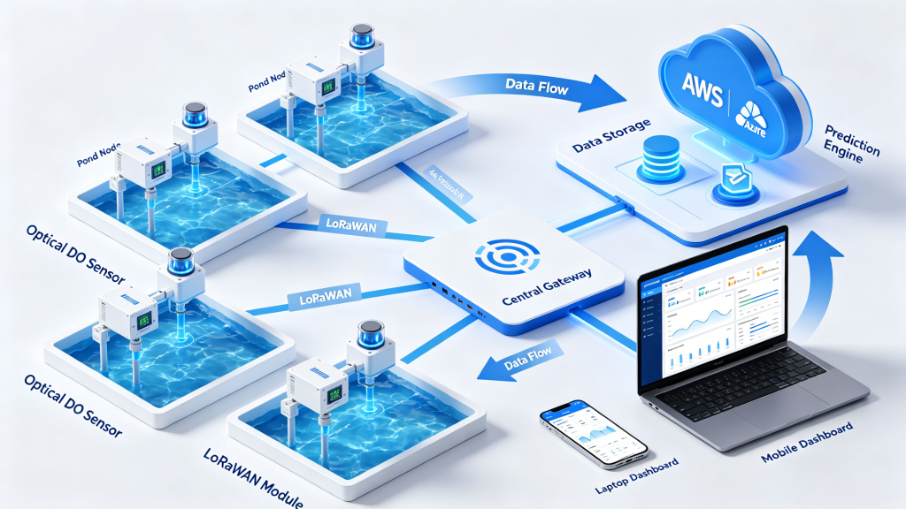
The tripartite enablers of intelligent DO management are: (i) low-power wide-area IoT sensors (e.g., LoRaWAN, NB-IoT, 4G/5G) providing reliable, high-frequency DO, temperature, and pH data; (ii) cloud platforms with scalable storage and real-time visualization dashboards; and (iii) AI/ML prediction engines running models from ARIMA to deep learning. These three layers form the backbone of any Industry 4.0 aquaculture system.

The Three Pillars of Dissolved Oxygen Prediction Modeling in Pond Aquaculture

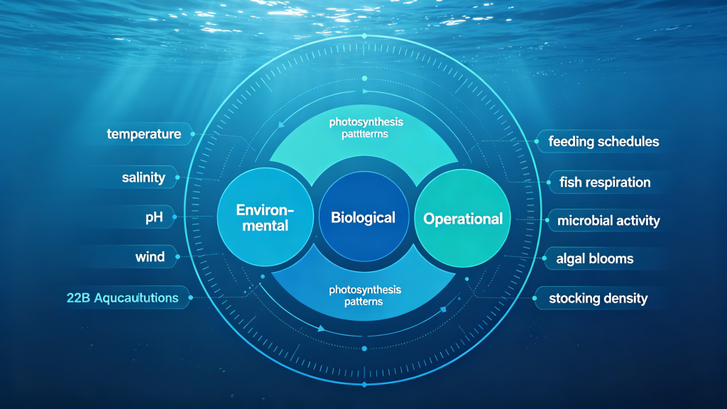
Driven Factors of DO: Environmental, biological, and operational influences

Temperature, salinity, pH, algal blooms, feeding schedules, aeration patterns

Dissolved oxygen concentration is governed by a complex interplay of direct and indirect factors. Direct factors include aeration input, photosynthetic oxygen production (by phytoplankton and submerged plants), and oxygen consumption by fish, bacteria, and sediment demand. Indirect factors encompass temperature (affects saturation concentration and metabolic rates), salinity (Henry’s law: higher salinity lowers oxygen solubility), pH (via algal bloom crash dynamics), and wind-induced mixing. Feeding schedules introduce periodic organic loads that stimulate microbial respiration, causing predictable DO dips 1–3 hours after feeding. Aeration patterns (location, duration, intensity) are the primary human intervention. Modern dissolved oxygen prediction modeling must incorporate all these drivers to achieve actionable accuracy.

Predictive Models: From statistics to deep learning

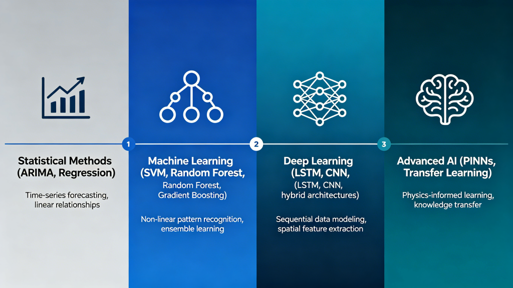
Statistical methods (ARIMA, regression) → Machine learning (SVM, random forest) → Deep learning (LSTM, CNN) → PINNs and transfer learning

The evolution of DO prediction mirrors the broader AI revolution. Statistical methods like ARIMA and multiple linear regression work well for steady-state, linear systems but fail to capture the nonlinearity of aquaculture DO. Machine learning approaches – Support Vector Machines (SVM), Random Forest (RF), and Gradient Boosting – model nonlinearities using feature engineering (lagged variables, rolling statistics). Field studies show RF often achieves R² 0.75–0.85. Deep learning, specifically Long Short-Term Memory (LSTM) networks, has become the gold standard for time-series DO prediction because LSTM explicitly learns long-term dependencies and temporal patterns (e.g., diurnal cycles). Convolutional Neural Networks (CNN) can extract local patterns, often combined with LSTM in hybrid architectures. For data-scarce environments, Physics-Informed Neural Networks (PINNs) embed the oxygen mass balance equation into the loss function, dramatically reducing data requirements. Transfer learning enables a model pre-trained on one farm to be fine-tuned with minimal local data (e.g., two weeks) for another farm, solving the “cold-start” problem.

Monitoring and Sensor Technologies: Electrochemical vs. optical with IoT integration

Two primary sensor technologies dominate commercial DO monitoring. Electrochemical (galvanic/polarographic) sensors are low-cost but require frequent calibration (every 2–4 weeks), membrane replacement, and suffer from drift. Optical sensors (fluorescence quenching) are more expensive upfront but offer long-term stability (calibration intervals of 6–12 months), faster response, and no oxygen consumption during measurement. For IoT integration, optical sensors pair better with low-power telemetry because they require less maintenance. Modern sensor nodes integrate with LoRaWAN or NB-IoT modules to transmit data to cloud platforms every 5–15 minutes.

DO Prediction Modeling Methods in Depth

Mechanistic modeling based on oxygen mass balance

Mechanistic (white-box) models rely on first-principles differential equations representing oxygen sources and sinks: dDO/dt = (kLa*(DOsat-DO) + P_photo – R_resp – BOD). While theoretically sound, they require difficult-to-measure parameters (volumetric mass transfer coefficient kLa, photosynthetic rate, sediment oxygen demand). Thus, pure mechanistic models are rarely deployed for real-time control but serve as the physical backbone for hybrid PINNs.

Machine learning approaches: SVM, random forest, gradient boosting

Ensemble tree-based methods like Random Forest and Gradient Boosting Machines (e.g., XGBoost, LightGBM) are favored by practitioners because they handle missing values, provide feature importance rankings, and are less prone to overfitting with moderate dataset sizes (3–6 months of hourly data). SVM with RBF kernels captures nonlinear boundaries but is less scalable to large data. Typical feature sets include DO at t-1, t-2, temperature, pH, salinity, aeration status, hour of day, and day of year. ML models often outperform deep learning on small datasets (fewer than 2000 samples).

Deep learning for time-series DO prediction: LSTM networks

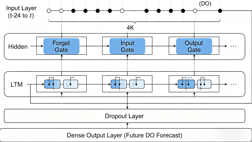
LSTM networks are specifically designed to learn long-term dependencies, making them ideal for DO prediction where past oxygen levels 12–24 hours ago influence current dynamics (e.g., morning DO trough after nocturnal respiration). A standard architecture includes an input layer (sequence length 12–24 time steps), two LSTM layers with 50–100 units each, dropout for regularization, and a dense output layer. Studies report LSTM achieving R² up to 0.94 and RMSE < 0.3 mg/L on high-frequency pond data. Variants like bidirectional LSTM and phased LSTM (which incorporates time gates) further improve performance by capturing both past and future context or irregular sampling.

Physics-informed neural networks (PINNs) for data-scarce environments

In many small-scale or new farms, historical data is insufficient for pure data-driven models. Physics-informed neural networks (PINNs) incorporate the oxygen mass balance differential equation as a soft constraint in the loss function. This reduces the required training data by up to 70%, while still respecting known physical laws. PINNs also improve extrapolation beyond observed ranges (e.g., extreme temperature spikes). Implementation requires automatic differentiation and is usually done in TensorFlow or PyTorch.

Transfer learning: Applying models across different farms

A major barrier to AI adoption is that every farm has unique characteristics. Transfer learning addresses this: pre-train a deep learning model (e.g., LSTM) on a large, publicly available dataset or on a donor farm with similar climate and species. Then fine-tune the last few layers using just 1–2 weeks of local data. Results show transfer learning achieves performance comparable to models trained from scratch with three months of data, accelerating deployment from months to days.

IoT-Based DO Monitoring and Control Systems for Dissolved Oxygen Prediction

Sensor network architecture: LoRaWAN, NB-IoT, 4G/5G

Selecting the right telemetry technology is critical for cost-effective, resilient monitoring. LoRaWAN offers ultra-low power (sensor battery life of 2–5 years) and long range (2–10 km in rural aquaculture ponds), but low bandwidth and higher latency; ideal for periodic DO data transmission (every 10–30 minutes). NB-IoT (Narrowband IoT) provides better penetration and lower latency, suitable for semi-real-time applications, but requires cellular coverage and carrier subscriptions. 4G/5G is used for video, edge processing, or high-frequency data (1-min intervals) but consumes more power. Most advanced farms deploy hybrid architectures: LoRaWAN for distributed pond sensors and 4G/5G gateways for cloud backhaul.

Cloud platforms for real-time data aggregation and visualization

A robust cloud platform (AWS IoT Core, Azure IoT Hub, or open-source alternatives like ThingsBoard) ingests streaming sensor data, applies validation rules, stores time-series data (e.g., InfluxDB), and provides interactive dashboards. Essential features include: multi-farm/pond views, historical trend analysis, alarm configurators, and API access for prediction models. Real-time dashboards enable farm managers to visualize predicted DO trajectories alongside actual measurements, building trust in AI recommendations.

Automated aeration control: Threshold-based, PID, and predictive control

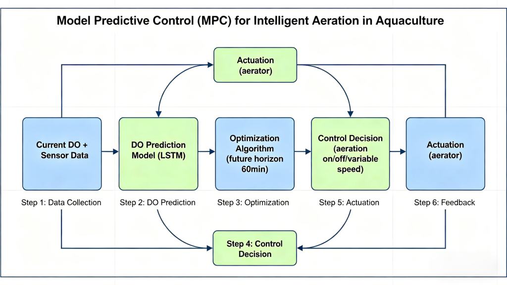
Control strategies form the final actuation layer. (i) Threshold-based control: simple on/off when DO falls below setpoint; simplest but inefficient and reactive. (ii) PID control: modulates aeration intensity proportionally to the error; smoother but still reactive. (iii) Predictive control (Model Predictive Control – MPC): uses DO prediction model to compute optimal aeration sequence over a future horizon (e.g., next 60 minutes), minimizing energy while keeping DO above threshold. MPC typically reduces energy use by an additional 10–15% compared to PID.

Mobile alerts and remote fleet management

Farm operators require immediate notification of impending hypoxia. Mobile apps (iOS/Android) push configurable alerts: predicted DO below 3 mg/L within 30 minutes, sensor disconnection, or aeration failure. Remote fleet management allows a single technician to oversee dozens of ponds via a centralized dashboard, adjust control parameters, and manually override automation when needed.

From Data to Action: Building a Complete Intelligent DO Management System

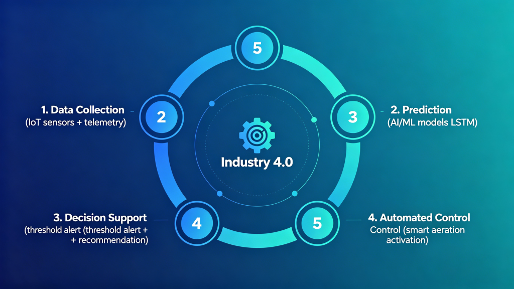
Data collection → Prediction → Decision support → Automated control → Feedback loop

End-to-end intelligent DO management follows a closed-loop cycle: 1) Data collection: optical DO sensors + temperature/pH probes transmit via LoRaWAN to cloud every 10 minutes. 2) Prediction: an LSTM or ensemble model forecasts DO for next 1–2 hours. 3) Decision support: if forecast drops below threshold, the system recommends aeration activation. 4) Automated control: cloud sends command to PLC or smart relay to turn on aerators. 5) Feedback loop: new DO measurements are ingested to retrain/update the model, improving accuracy daily. This “sense-predict-act-learn” loop embodies Industry 4.0’s cyber-physical systems.

Case study: 97.74% accuracy in IoT-based brackish water shrimp farming

A documented commercial deployment (2024-2025) in a 50-hectare brackish water shrimp farm integrated optical DO sensors, LoRaWAN gateways, and a hybrid CNN-LSTM prediction model. The model was trained on 4 months of hourly data (DO, temperature, salinity, pH, aeration status). After optimization, the system achieved 97.74% prediction accuracy (defined as predicted DO within ±0.5 mg/L of actual value, 30-minute horizon). The predictive control reduced aeration runtime by 26% while maintaining DO above 4 mg/L during critical night hours. Shrimp survival rate increased by 8% compared to the previous season, and feed conversion improved by 9%. This case demonstrates that triple-digit ROI is achievable within one season.

Frequently Asked Questions About DO Prediction and Control

What is the minimum data required to build a DO prediction model?

Typically 3–6 months of hourly data including DO, temperature, and aeration status. For deep learning (LSTM), 6 months is recommended; for random forest, 3 months may suffice. If using PINNs or transfer learning, as little as 2–4 weeks of local data can be adequate when combined with pre-trained models or physical constraints.

Can DO prediction models be transferred between different farms?

Yes, using transfer learning techniques. Pre-train a model (e.g., LSTM) on one farm’s data, then fine-tune on the target farm with only 1–2 weeks of local data. Works best if farms share similar climate, species, and aeration systems. This approach reduces deployment cost and accelerates ROI.

What is the ROI of implementing AI-based DO control vs. traditional aeration?

Meta-analysis of multiple studies shows 15–30% energy savings from predictive aeration, plus 5–10% FCR improvement and 2–8% mortality reduction. For a middle-sized farm (USD 500k annual operating cost), ROI often exceeds 40% within the first year, excluding intangibles like reduced labor and better regulatory compliance.

Do I need an on-premises server or cloud connectivity?

Most modern solutions operate on cloud platforms (AWS, Azure, or specialized aquatech clouds) requiring internet connectivity. Edge computing alternatives exist for remote farms: a local gateway runs lightweight models (e.g., TinyML on Raspberry Pi or Jetson Nano) and only syncs summary data to cloud when bandwidth is available. Hybrid edge-cloud architectures are becoming standard.

Which model performs best for real-time control – LSTM or Random Forest?

For real-time control with high-frequency data (>1 sample/10min) and long sequences, LSTM generally outperforms (lower RMSE). However, Random Forest is simpler to implement, interpretable (feature importance), and faster to train; it remains a robust choice for farms with < 2000 samples. Many engineers start with RF as a benchmark before moving to LSTM.

What sensors are recommended for long-term IoT deployment?

Optical (fluorescence) DO sensors are preferred for long-term unattended operation due to drift-free performance (6-12 months calibration interval) and no oxygen consumption. Pair them with a temperature probe and optional pH/salinity sensors. Select telemetry (LoRaWAN vs NB-IoT) based on farm area and cellular coverage.