Step-by-Step Guide for Engineers: How to Build Your Own DO Prediction Model

Building a DO prediction model is a transformative engineering task that enables proactive management of dissolved oxygen in aquaculture, wastewater treatment, and environmental monitoring. This step-by-step guide compiles the most authoritative methodologies to help you construct a reliable predictive system from scratch.

Dissolved oxygen (DO) is a critical water quality parameter. Accurate DO prediction model development allows you to anticipate changes before they occur, reducing energy costs, preventing fish kills, and ensuring regulatory compliance. While real-time DO sensors are essential, a predictive model transforms your operation from reactive to proactive.

Why Build a DO Prediction Model? The Engineering Imperative

Traditional DO monitoring is reactive—you only know oxygen levels after they drop. A DO prediction model shifts your operation to proactive management. Key benefits include:

Energy Optimization: In aeration systems, predicting low DO allows preemptive aeration rate adjustments, reducing electricity consumption by up to 30%.
Fish Health Protection: In aquaculture, early warning of hypoxic events prevents mass mortality and reduces stress-induced disease.
Process Control: In wastewater treatment, accurate predictions optimize biological treatment efficiency and prevent sludge bulking.
Regulatory Compliance: Continuous prediction helps avoid permit violations by ensuring DO never falls below mandated thresholds.

The core principle is that DO is not random; it follows patterns driven by physical, chemical, and biological factors. Your DO prediction model will learn these patterns.

DO prediction model engineering overview showing sensor data and predictive analytics

Step 1: Understand the Key Influencing Factors

A successful DO prediction model begins with understanding what drives oxygen dynamics. Based on the most authoritative sources, the primary variables you must collect data for are:

Physical Factors

Water Temperature: The single most influential factor. Cold water holds more oxygen. Temperature inversely correlates with DO saturation.
Salinity: Higher salinity reduces oxygen solubility. Critical for marine or brackish water applications.
Atmospheric Pressure: Lower pressure (e.g., high altitude) reduces DO saturation. Barometric pressure data improves model accuracy.
Turbidity & Light Intensity: In photosynthetic systems (e.g., ponds, lakes), light drives oxygen production. Turbidity reduces light penetration, limiting photosynthesis.

Biological & Chemical Factors

Biochemical Oxygen Demand (BOD) / Chemical Oxygen Demand (COD): Measures of organic pollution. High BOD leads to rapid oxygen consumption.
Chlorophyll-a (Algae Density): A proxy for photosynthetic oxygen production. High algae can cause extreme diurnal DO swings.
Ammonia & Nitrite: Indicators of biological activity that consume oxygen during nitrification.
Fish Biomass / Feeding Rate: In aquaculture, fish respiration and uneaten feed decomposition are major oxygen sinks.

Operational Factors (for Controlled Systems)

Aeration Rate (Oxygen Transfer): The most controllable variable. Record airflow rates, diffuser depth, and aeration schedules.
Water Exchange Rate: Inflow of fresh water introduces new oxygen.
Depth: DO can vary significantly with depth due to stratification.

Data Collection Mandate: You must log these variables at a consistent interval (e.g., every 10–60 minutes). Historical data spanning at least one full seasonal cycle (ideally 12+ months) is required for robust model training.

DO sensor data collection in aquaculture for prediction model

Step 2: Choose Your Modeling Approach

Based on the most comprehensive engineering literature, there are three primary approaches for your DO prediction model. Your choice depends on data availability, computational resources, and desired accuracy.

Approach A: Data-Driven Machine Learning (ML) Models

This is the most popular and powerful method for modern engineers. ML models learn complex, non-linear relationships without requiring explicit physical equations.

Best For: Systems with abundant historical sensor data (temperature, DO, aeration, etc.).
Algorithms to Consider:
- Artificial Neural Networks (ANNs): Excellent for capturing non-linear dynamics. A feedforward backpropagation network with one or two hidden layers is a strong starting point.
- Long Short-Term Memory (LSTM) Networks: A type of recurrent neural network (RNN) specifically designed for time-series forecasting. LSTMs “remember” long-term dependencies, making them ideal for predicting DO based on past sequences (e.g., last 24 hours of data).
- Random Forest (RF) & Gradient Boosting (XGBoost): Robust, interpretable models that handle missing data well. They are faster to train than neural networks and provide feature importance rankings.
Key Advantage: No need to know the underlying physics of oxygen transfer. The model learns from data alone.
Key Challenge: Requires large, high-quality datasets. Prone to overfitting if not properly validated.

Approach B: Hybrid Physics-Based Models

This approach combines fundamental mass-balance equations with data-driven parameter estimation. It is more complex but highly interpretable.

Best For: Engineers who understand the physical processes and need a model that can extrapolate beyond the training data range.
How It Works:
1. Write the Mass Balance Equation: \( dDO/dt = K_L a (DO_{sat} – DO) + P – R \)
2. Estimate Parameters from Data: Instead of guessing \( K_L a \) or \( R \), use your historical data to fit these parameters using regression or optimization algorithms.
Key Advantage: The model is grounded in real physics, making it more robust to sudden changes in system operation.
Key Challenge: Requires deep domain knowledge and careful calibration. Can be difficult to implement for complex systems.

Approach C: Simple Statistical Regression

This is the simplest approach, suitable for quick estimates with minimal data.

Best For: Preliminary analysis or systems with very stable conditions.
How It Works: Use multiple linear regression (MLR) to model DO as a function of temperature, aeration, and time of day.
Key Limitation: Fails to capture non-linear dynamics and time-lag effects. Not recommended for critical applications.

Recommendation: For most B2B engineers seeking high accuracy and automation, start with LSTM networks (for time-series data) or Random Forest (for tabular sensor data). If you have a strong grasp of the system’s physics, the hybrid approach offers the best of both worlds.

LSTM neural network architecture for DO prediction model

Step 3: Data Preprocessing & Feature Engineering

This step is often the most time-consuming but is critical for your DO prediction model success. Garbage in = garbage out.

1. Handle Missing Data

Interpolation: For short gaps (< 1 hour), use linear interpolation.
Forward/Backward Fill: For sensor dropouts, fill with the last known value.
Remove: If a large chunk of data is missing (e.g., > 20% of a day), remove that period entirely.

2. Remove Outliers

Physical Limits: Flag any DO value > 20 mg/L or < 0 mg/L as erroneous.
Statistical Limits: Use a rolling z-score (e.g., remove points > 3 standard deviations from a 24-hour moving window). Sensor spikes due to cleaning or biofouling must be removed.

3. Create Lag Features (Crucial for Time-Series)

DO at time *t* depends on conditions at time *t-1, t-2, … t-n*. Create new columns:

DO_lag_1h: DO value from 1 hour ago.
Temperature_lag_2h: Temperature from 2 hours ago.
Aeration_lag_30min: Aeration rate from 30 minutes ago.
Domain-Specific Lags: In aquaculture, a feeding event may affect DO 2 hours later. Create a lagged feeding indicator.

4. Create Rolling Window Features

DO_rolling_mean_6h: Average DO over the last 6 hours.
Temperature_rolling_std_24h: Temperature variability over the last day.
Aeration_rolling_sum_12h: Total aeration energy over the last half-day.

5. Normalize/Standardize Data

ML algorithms perform better when all features are on a similar scale.

Min-Max Scaling: Scale values to [0, 1].
Z-Score Standardization: Center data around mean 0 with standard deviation 1. Preferred for neural networks.

Step 4: Model Training & Validation

Split Your Data

Training Set: 70% of data (oldest chronological data).
Validation Set: 15% (used to tune hyperparameters).
Test Set: 15% (newest data, never seen by the model). This is your final accuracy benchmark.

Train the Model

For LSTM: Define the sequence length (e.g., 48 timesteps = 48 hours of history). Use a Keras or PyTorch framework. Start with 1–2 LSTM layers, 50–100 units each, followed by a dense output layer. Use Mean Squared Error (MSE) as the loss function.
For Random Forest: Set the number of trees (n_estimators) to 500–1000. Use default settings initially, then tune max_depth and min_samples_leaf.

Validate Rigorously

Time-Series Cross-Validation: Do NOT use random k-fold cross-validation. It will leak future information into the past. Use expanding window or sliding window cross-validation.
Metrics to Track:
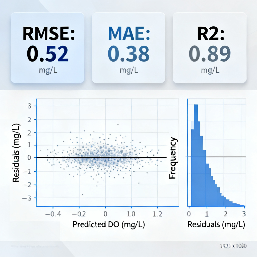
- Root Mean Squared Error (RMSE): Most common. In the same units as DO (mg/L). An RMSE < 0.5 mg/L is excellent.
- Mean Absolute Error (MAE): Less sensitive to outliers.
- R² (Coefficient of Determination): How much variance is explained. > 0.85 is good.
- Residual Analysis: Plot predicted vs. actual values. Look for systematic biases (e.g., model always overpredicts at low DO).

DO prediction model validation metrics and error analysis

Step 5: Deployment & Integration with Sensor Systems

A DO prediction model is only useful if it runs in real-time. Here’s how to bridge the gap from development to operational use.

Real-Time Data Pipeline

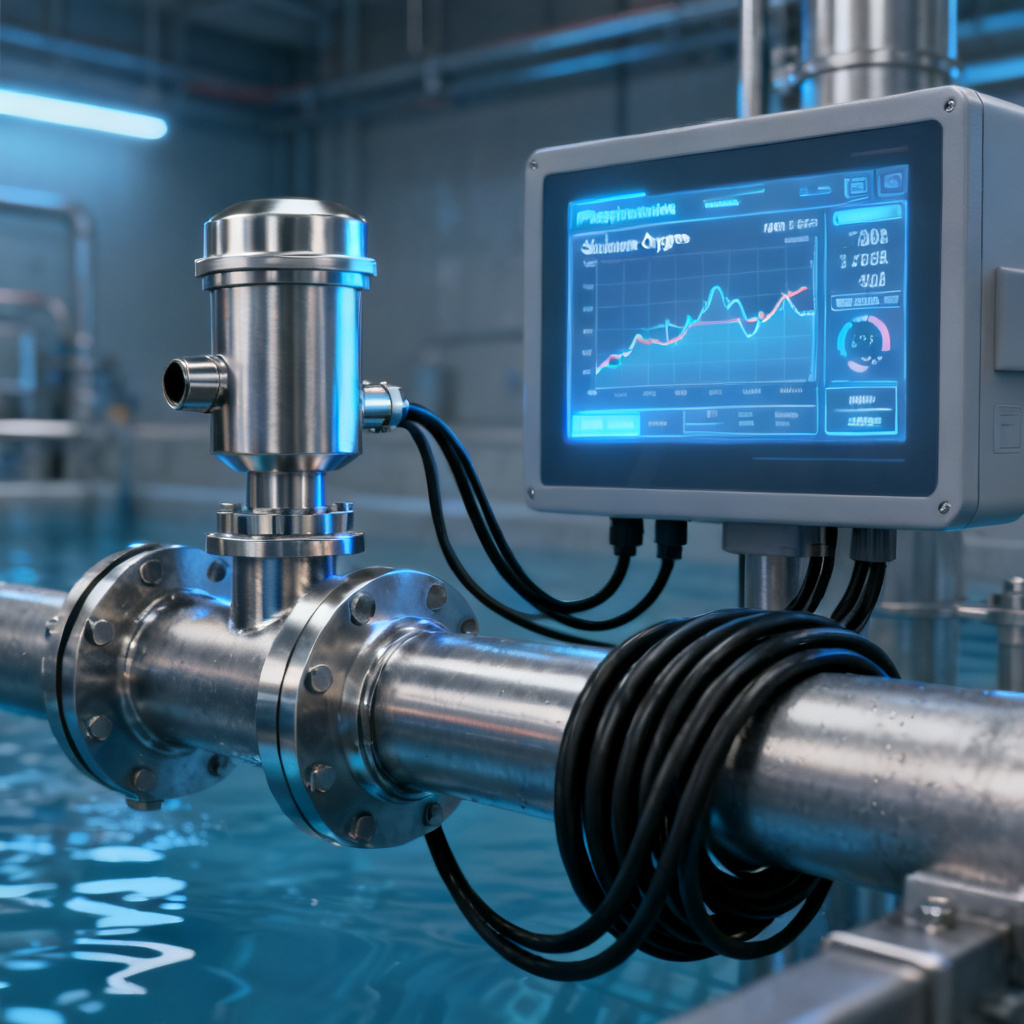
Sensor Data Ingestion: Your DO sensor, temperature probe, and other instruments (e.g., via Modbus, 4-20mA, SDI-12) send data to a PLC or edge gateway.
Data Cleaning: The gateway runs your preprocessing script (outlier removal, lag creation) in real-time.
Model Inference: The cleaned, formatted data is fed into your trained model (loaded as a .h5 file for LSTM or .pkl for Random Forest).
Output: The model outputs the predicted DO for the next 1, 6, or 24 hours.

Implementation Options

Edge Computing: Run the model directly on a Raspberry Pi, Jetson Nano, or industrial IoT gateway. This is ideal for remote sites with limited internet. The edge device can control aerators locally based on predictions.
Cloud-Based: Send data to AWS, Azure, or Google Cloud. Run the model on a server. This allows for more complex models and centralized dashboards. Latency must be acceptable for your control needs.

Actionable Alerts & Control

Predictive Alarms: If predicted DO drops below 3 mg/L in 2 hours, send an SMS or email alert.
Automatic Aeration Control: If the model predicts a DO deficit, the PLC automatically increases the aeration rate before the DO actually drops. This is the holy grail of energy savings.

Step 6: Model Maintenance & Retraining

DO dynamics change over time. Sensor drift, seasonal shifts, and system modifications (e.g., new aerators, different feed) degrade your DO prediction model accuracy.

Monitor Prediction Error: Continuously track the MAE between predicted and actual DO. If MAE exceeds a threshold (e.g., > 0.8 mg/L for 7 consecutive days), trigger a retraining event.
Retraining Schedule:
- Incremental Learning: Update the model daily or weekly with new data. This is computationally cheap.
- Full Retraining: Every 3–6 months, retrain the entire model from scratch using all accumulated data. This prevents concept drift.
Sensor Calibration: Your model is only as good as your sensors. Calibrate your DO sensor every 1–2 months (or per manufacturer specs). Log calibration dates—a sudden increase in prediction error often coincides with sensor fouling or calibration drift.

Common Pitfalls & How to Avoid Them

Pitfall	Solution
Ignoring Time Dynamics	Always use lag features or LSTM.
Overfitting to Seasonal Patterns	Include at least one full year of data.
Using Random Cross-Validation	Use time-series cross-validation.
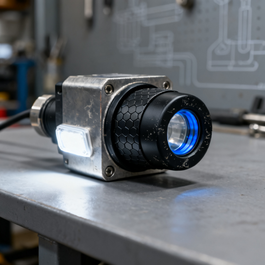
Neglecting Sensor Quality	Invest in reliable, industrial-grade optical DO sensors.
Thinking One Model Fits All	Build separate models for each distinct water body or process unit.

Frequently Asked Questions about DO Prediction Models

What is a DO prediction model and why do I need one?

A DO prediction model is a mathematical or machine learning tool that forecasts future dissolved oxygen levels based on historical data and current conditions. You need one to transition from reactive to proactive water quality management, saving energy and protecting aquatic life.

How long does it take to build a DO prediction model?

Building a robust DO prediction model typically takes 2–6 months, depending on data availability, model complexity, and deployment requirements. The most time-consuming phase is data collection and preprocessing.

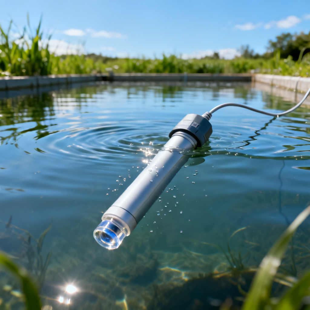
What sensors are required for a DO prediction model?

Essential sensors include a reliable dissolved oxygen sensor, temperature probe, and aeration rate monitor. Additional sensors for salinity, pressure, turbidity, and BOD can improve model accuracy in specific applications.

Can I use a DO prediction model with existing sensor infrastructure?

Yes. Most DO prediction models are designed to integrate with existing PLCs, SCADA systems, or IoT gateways via standard protocols like Modbus, 4-20mA, or SDI-12. No need to replace your entire sensor network.

How often should I retrain my DO prediction model?

Retrain your DO prediction model every 3–6 months or whenever prediction error exceeds your threshold (e.g., MAE > 0.8 mg/L for 7 consecutive days). Incremental updates can be done weekly for continuous improvement.

Conclusion: From Data to Decision

Building your own DO prediction model is a multi-step engineering process that combines sensor technology, data science, and domain expertise. By systematically collecting the right variables, choosing an appropriate algorithm (LSTM for time-series or hybrid physics-based for robustness), rigorously validating with time-series cross-validation, and deploying on an edge or cloud platform, you can transform raw sensor data into actionable intelligence.

The result is not just a model—it is a decision-support system that saves energy, protects aquatic life, and optimizes your entire process. Start with your data, build incrementally, and refine continuously. Your DO sensor is the eyes; your DO prediction model is the brain. Together, they make your system truly intelligent.

Need a reliable foundation for your prediction model? Our industrial-grade optical dissolved oxygen sensors provide the stable, drift-free data that accurate prediction requires. Contact us to discuss how our sensors and custom calibration services can support your next engineering project.